Article
Bad Excel Habits and How to Fix Them
Avoiding these bad habits will make it easier for others to work with your spreadsheets and make it easier for you to update and maintain them.
- Mixing Data with Reporting and Calculations
- Missing Values
- Inconsistent Values
- Storing Multiple Things in a Single Column
- Ambiguous Dates and Times
- Using Only Colors or Icons to Represent Information
- Extensive Formatting
- Not Using Aliases in Formulas
Mixing Data with Reporting and Calculations
Spreadsheet tools like Excel and Google Docs are versatile and they make it easy to mix everything together on one sheet for quick analysis. However, if everything is mixed on a single sheet and you change the data in-place, it will be harder to reproduce and update with new/additional data in the future.
By clearly separating the data from everything else it will be easier to update and maintain, and you'll also have a good source of data to export for use in other tools.
Here's some clarification of what I mean when I say data, calculations, and reporting:
Data - raw and unprocessed, exactly how it first arrives to the spreadsheet/workbook, whether it's being typed in via manual data entry or imported from a database.
Calculations - anything done to the original data after it's initial import into the spreadsheet. This can include how you split the data into different sheets.
Reporting - can range from summary tables with subtotals and pivots to visualizations like charts and graphs.
Some warning signs of mixing:
- Blank rows or subtotals in the middle of a data sheet
- Columns change type/name/formula partway down a data sheet
- Extensive formatting of a data sheet (see below)
- Using sheetname as another column (e.g. 'jan', 'feb', 'mar')
Fixing it
- Remove blank rows, and move (sub)totals to a reporting sheet
- Columns that change part-way down the sheet indicate a different type of data: separate the two types of data, each on it's own data sheet
- Combine data sheets that differ only by sheetname and create a column for the old sheetnames (e.g. combine monthly sheets into a single sheet with a column for month, now it's easy report on quarterly and yearly numbers too)
A well-structured collection of spreadsheets will allow you to append rows to the bottom of data sheet(s) without destroying calculations and reporting.
In my opinion, this is the most important bad habit listed in this article. If you invest any time in correcting some of the bad habits described here, start here with separating data cleanly!
Missing Values
Not differentiating between a missing value and a true zero or False can lead to confusion later.
How you represent missing values is also important. Consistency is most critical but
another thing to consider is compatibility with other software you might want to
import this data into. Avoid representing missing data with numbers like 0 or -999,
especially in columns of numbers. NULL is good for SQL databases and NA (as
in 'not applicable' or 'not available') is also a good choice. As long as you are
consistent, you can always do a find and replace later.
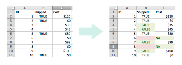
The two sheets above illustrate the problem with blank cells and using numbers like 0 as markers for missing data. The sheet on the left omits FALSE values in the Shipped column, making it impossible to tell if an empty cell in that column indicates shipped = False or if nobody has calculated what it should be. With the formatting of the sheet on the right, it's easy to see that the rows with id 6 and 8 are yet to be calculated or were accidently cleared. The updated formatting of the sheet on the right also reveals that 0's were being used to mark missing data in two rows of the Cost column.
Inconsistent Values
Autocomplete is your friend in this regard, but can be flakey, especially on larger sheets and if there are blank rows in the column.
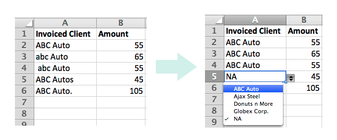
The fix is to use Excel's data validation feature, with it, you can enforce consistent allowable values in a row or column including choosing from a set of known options. This can increase the speed of data entry as well as reduce the need for fuzzy matching later on.
Storing Multiple Things in a Single Column
Very common, and easily fixed. Example:
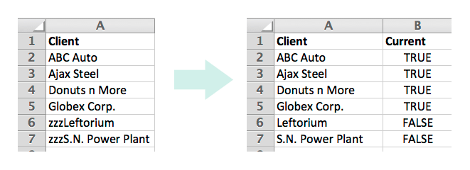
zzCustomer Name in which zz is prepended to existing values as a flag to indicate
something else, like that they are no longer active. It's often prepended so users can
sort by the new dimension.
The solution is to be diligent about breaking out that additional information into a separate column. You can still filter and sort using the new column.
Ambiguous Dates and Times
A whole article could be devoted to dealing with dates and times in Excel. What you see in an open Excel-sheet is often not what is saved to file or exported. It can depend on the format of the cells and your computer's "Region" settings and probably other things I'm not aware of. Here's an incomplete list of things to keep in mind:
- Consistency is key, again.
- Watch out for ambiguous formats like
04/05/06in which any of the numbers could indicate the year. Four digit years will help, even better is using a well known and standardized format like ISO 8601, which is possible with a custom format applied to cellsyyyy-mm-ddThh:MM:ss. But again, these date formats might not be what is saved when you export to csv, unless you convert the cells to typetextfirst - If you are including times, you should include timezone; if no timezone is there,
I, and some tools will assume it is
UTC (+00). However, Excel
has no time zone format! One way to include time zone data is to store it in another
column separately, e.g.
EDTor-04:00and ensure it's formatted to be text.
Solution: Keep your original date column, formatted the way you like to look at them
and the way you like to input them, but add another date/time column and format the
cells in it as text (so they will be exported in a predictable format). In the
text-based date column apply the formula =TEXT(A1,"yyyy-mm-ddThh:MM:ss") in which
A is the column containing your ambiguously formatted dates.
Using Only Colors or Icons to Represent Information
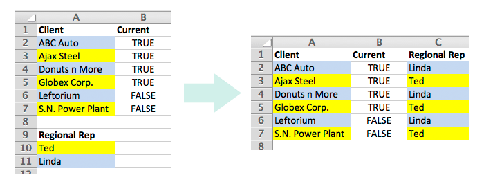
While recent versions of Excel will allow you to sort and filter by color or icon this information will likely be lost when importing the excel file into another tool.
The fix is easy, just make another column (hide it if necessary) and have it's values be what the colors represent. You can even keep your colors and use the new column as the basis for a formula to apply colors automatically using conditional formatting too.
Extensive Formatting
Merged cells, blank lines, subtotals, colors that mean something; all of these things will present problems when trying to read Excel data into another program or database. They also encourage other bad habits, e.g. if the sheet's complex formatting breaks when adding a new column it is far more tempting to smush two (or more!) pieces of info into a single cell.
The Formatting problems mentioned in this section and the colors/icons section above are probably only an issue if they are applied to a data sheet. If you have successfully separated the reporting and calculations from the data in a workbook, it is most likely ok to make the reporting sheet(s) look nice with merged cells, etc.
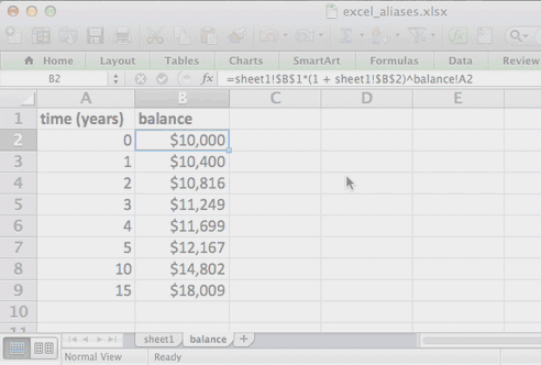
Not Using Aliases in Formulas
Instead of referencing a cell with sheet1!$B$1 you can use profit. See the
Microsoft documentation.
This is a big time saver for anyone (including yourself a year from now) that has to figure out how the formulas in a sheet work. The demo below is simplified, but this becomes much more helpful when converting elaborate dashboards from Excel to another tool.
Note* it's not obvious how to update the range of cells in a named range like
'year' in the above example: if you see a "name manager" icon in the formula tab of
the ribbon you can edit a defined name to change the range it applies to. If you
don't see that button in your version of Excel you can find something similar in
Insert -> Name -> Define....
References:
- Sort and filter by color: https://support.office.com/en-us/article/Guidelines-and-examples-for-sorting-and-filtering-data-by-color-b1bf3982-051d-49b8-8330-80e99c94365b
- select and treat all blank cells: http://www.contextures.com/xlDataEntry02.html
- data carpentry spreadsheet mistakes: http://www.datacarpentry.org/2015-03-09-ISI-CODATA/lessons/excel/ecology-examples/02-common-mistakes.html
- summary on why using Excel for ETL and as as database is a bad idea: http://datascience.stackexchange.com/a/5450
- top 10 on bad spreadsheet design: http://www.techrepublic.com/blog/10-things/10-ways-to-screw-up-your-spreadsheet-design/
- seven deadly sins of data entry article: http://datascopic.net/xlcaliber-7deadlysins/?doing_wp_cron=1486052766.4989480972290039062500
- tek-tips deadly Excel habits: http://www.tek-tips.com/viewthread.cfm?qid=1525860
- spreadsheet worst practices from CFO perspective: http://ww2.cfo.com/technology/2008/05/spreadsheet-worst-practices/
- python Excel tutorial: the definitive guide (datacamp): https://www.datacamp.com/community/tutorials/python-excel-tutorial#gs.Hz1IdX0
- python packages to work with Excel files in python: http://www.python-excel.org
- Enthought's article of fundamental problems with Excel: http://blog.enthought.com/general/avoiding-excel-hell-using-a-python-based-toolchain/#.WI9yYOlRRRF
- Enthought's slides on problems with Excel: http://blog.enthought.com/wp-content/uploads/QPUG_20130514_ExcelHell_Slides.pdf